The Passenger Transfer Efficiency Coefficient (PTEC) for Double Deck Elevators under Incoming Traffic Conditions
Lutfi Al-Sharif , Enas AlOsta, Noor Abualhomos, Yazan Suhweil
Mechatronics Engineering Department, School of Engineering
The University of Jordan, Amman 11942, Jordan
This paper was presented at The 7th Symposium on Lift & Escalator Technology (CIBSE Lifts Group and The University of Northampton) (2017). This web version © Peters Research Ltd 2019.
Keywords: Elevator, lift, high rise buildings, double deck elevator, round trip time, up-peak traffic, incoming traffic, Monte Carlo Simulation.
Abstract. One of the sources of efficiency in the operation of double deck elevators is the simultaneous transfer of passengers into and out of the elevator cars, thus leading to a reduction in the value of the round trip time, and thus an increase in the handling capacity.
However, due to the randomness of passenger destination selections, this reduction is not optimal. This paper presents this phenomenon as an efficiency coefficient, denoted as the Passenger Transfer Efficiency Coefficient (PTEC) and is representative of the time taken by passenger to alight from the double deck elevator.
PTEC is mainly applicable to passengers alighting, rather than passengers boarding. This is true in the case of a single pair of entrances. For the case of multiple pairs of entrances, the PTEC applies to both alighting and boarding operations.
A set of equations are derived in order to calculate the PTEC. The results from the equations are verified using the Monte Carlo simulation method. The method of stepwise verification has been used in order to verify the equations.
Nomenclature
L the number of elevators in the group
N the total number of floors above the pair of main entrances
P the number of passengers per deck
Pe the number of passengers for the even deck
Po the number of passengers for the odd deck
PTEC passenger transfer efficiency coefficient
S is the expected value of the number of stops in a round trip
tp the passenger alighting or boarding time in seconds
U is the total building population in persons
Ui is the population of the ith floor in persons
Ue is the total population of the even floors in persons
Uo is the total population of the odd floors in persons
1 Introduction
Double deck elevators offer a very efficient means of moving people within buildings ([1], [2] and [3]). By placing two conventional single deck elevators one on top of the other and attaching them rigidly, shaft space is saved. Passengers board both decks at the same time, whereby passengers heading to an odd floor board the lower deck and passenger heading to the even floors board the upper deck. The elevator then moves two floors at a time. Once a stop is made, passengers alight simultaneously from the upper and lower decks to the even and odd destination floors respectively.
There are three sources of efficiency that arise from using double deck elevators:
- The effective number of stops is reduced due to the fact that the potential number of floors is halved (N/2 instead of N). This reduces the value of the round trip time and thus increases the handling capacity.
- The passenger boarding and alighting time is reduced due to simultaneous boarding and alighting of passengers on the two decks.
- Due to the fact that the two elevator cars are mounted on top of each other, the car capacity is increased without a major increase in the core space usage.
Double deck elevators are mainly used in two broad applications ([4], [5]):
- They are effective as shuttles between the ground floor and sky lobbies. The efficiency arises from the fact that there are only two stops (or three stops) thus reducing the value of the round trip time. The elevator car capacity in such situations is made relatively large.
- They are currently increasingly being used in low and medium rise buildings in cases where the floor populations are relatively high. For example, double deck elevators can be very effective in buildings with more than 250 persons per floor (examples are given in [6]).
Barney [4] presents a comprehensive list of the double decker installation around the world and their applications. Siikonen [7] presents the equations for the expected number of stops (S) and the highest reversal floor (H) for the case of equal and unequal populations and derives a parameter for the passenger transfer efficiency. Genetic algorithms have been widely applied in elevator traffic control systems examples of which can be found in ([7], [9], [10] and [11]). More specifically, Sorsa et al. [8] use genetic algorithms to achieve optimal control of double deck elevators.
Two pieces of work on double deck elevator formulae are given by Kavounas [12] and Peters [13] and [14]. Kavounas derives a formula for the highest reversal floor and the expected number of stops. Peters [13] and [14] presents formulae for the general case under Poisson arrival conditions. However, it is difficult to carry out comparison with the results in these papers as they do not present any closed form equations (instead, calculations that they present are iterative and require computer implementation).
The published research in the area of double deck elevator does not address the following two points:
- No mathematical formula has been derived for the passenger transfer efficiency (i.e., the quantification of the benefits of simultaneous passenger alighting at the destination floors). The main aim of this paper is to derive a formula for the passenger transfer efficiency. This is critical in enabling the correct calculation of the round trip time ([15], [16], [17]).
- No verification has been carried out to ensure the accuracy of the derived equations. The derived equations presented in this paper have been verified using the Monte Carlo Simulation method (MCS).
Section 2 introduces some necessary assumptions and numbering conventions used in this paper. Section 3 introduces the concept of the passenger transfer efficiency and derives equations for the PTEC for the cases of equal floor populations. Section 4 discusses a similar parameter presented by Siikonen. Section 5 presents a numerical example to understand the effect of the number of passengers, P, and the number of floors, N, on the coefficient. Conclusions are drawn in section 6.
2 Assumptions and numbering conventions
In this section some of the assumptions are clearly stated as well as the numbering notation for the building. It is necessary to clearly state some of the assumptions that will be made within this paper and provide some background required for the derivations.
Throughout this paper, it will be assumed that a single pair of entrances is used for boarding. There is only one pair of entrance floor, which is in effect a single entrance scenario. Each passenger can only enter the building through one floor: the odd entrance for odd destination occupant floors and the even entrance for even destination occupant floors.
It will also be assumed that all traffic is incoming traffic. Incoming traffic is traffic that originates at an entrance floor and terminates at an occupant floor. This is not an unreasonable assumption to make. The reason for this is that double deck elevators are usually operated in double deck mode under incoming traffic conditions during which they are most efficient. The design of double deck elevators is still based on the morning incoming traffic (up peak traffic). It is usual to operated double deck elevators in single deck mode outside peak hours. Under single deck mode, one of the decks is deactivated and the other deck serves passengers as a single deck.
It is also necessary to define the concept of a twin pair of floors, one of which is odd and the other even. This concept is critical to all the derivations that will follow in this paper. A twin pair of floors is, as the name implies, consecutive floors at which the double deck will make a simultaneous stop and deliver passengers. For brevity in the analysis below, the pair of twin floors will be simply referred to as twin floors. The lower floor will be assumed to be the odd floor and given the subscript o for odd; the upper floor will be assumed to be the even floor and given the subscript e for even. A general overview of the arrangement of a building that is served by double deck elevators is shown in Figure 1.
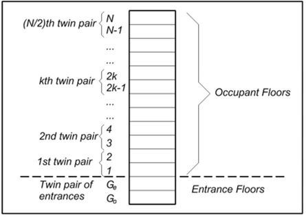
Figure 1: General overview of a building served by double deck elevators, showing the numbering convention used.
It will also be assumed that the number of occupant floors is even. This is the most efficient arrangement. However, some notes are given in [18] as to how the case of an odd number of occupant floors can be addressed.
3 Derivation of the formula for the Passenger Transfer efficiency coefficient
The passenger transfer efficiency coefficient (PTEC) is unique to double deck elevator systems (or to multiple deck systems in general). It is a measure of the efficiency of the passenger transfer time (i.e., boarding and alighting). There are two phases of passenger transfer in any elevator: boarding time and alighting time.
Based on a single pair of entrances, passenger transfer efficiency during boarding is not a concern (noting that it is assumed that all the traffic is incoming only). It is assumed that all P passengers for each deck (i.e., the upper deck and the lower deck) start boarding at the same time and finish boarding at the same time. Thus there is no wasted time and full efficiency is automatically attained.
However, the issue of passenger transfer efficiency is more of a concern during alighting. As there are many occupant pairs of floors (that will act as destinations for passengers) it is likely that different numbers of passengers are destined for the odd and even floors of the same stop. The most efficient scenario would take place in a double deck elevator when an equal number of passengers from the two decks alight at the same stop. In this case it can be stated that there is no wasted time, as there is no wasted waiting time at one deck while one or more passengers are alighting from the other deck.
For example, if at one of the double decker stops, five passengers alight from the upper (even) deck and one passenger alights from the lower (odd) deck, then the actual alighting time is equal to the time required for the five passenger to alight from the upper deck. The difference between the numbers of passengers intending to alight at this stop has effectively caused a loss of time. Had the number of passengers intending to alight been equal (i.e., three passengers for the upper deck and the three passengers for the lower deck) then the total alighting time would have been only equal to the time required for three passengers to alight, resulting in a saving equal to the time required by two passengers to alight. It is this efficiency (or inefficiency) that this parameters aims to capture. The formula for the case of equal floor population will be derived in this section.
In order to derive a formula for the PTEC, it is necessary to find an expression for the probability of the number passengers destined for the odd floor of the twin pair of floors being equal to i and the passengers destined for the even floor of the twin pair of floors being equal to j.
Each of these events shall be denoted as A and B respectively, as follow:
A is the event under which i passengers are destined for the odd floor of the pair of twin floors.
B is the event under which j passengers are destined for the even floor of the pair of twin floors.
For each of these events, the probability distribution function is effectively a binomial distribution (i.e., a passenger can either head or not to a certain floor). For each deck, it is assumed that P passengers will board the deck in each round trip at the main entrance.
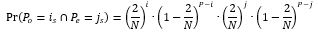
It is now necessary to find the probability of i specific passengers going to a floor. This implies that other P-i passenger did not go to that floor. The probability of the joint event is the product of the two probabilities:
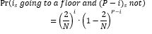 (1)
(1)
This can then be applied to the odd floor of the twin floors and the even floor of the twin floors as shown in the two equations below. (It is implied that if i specific passengers go the floor then P-i passengers will not without the need to explicitly state it in the formula).
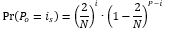 (2)
(2)
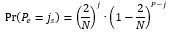 (3)
(3)
As the two events are independent, then the combined event whereby i specific passengers head to the odd floor and j specific passengers head to the even floor of the twin pair of floors is:
 (4)
(4)
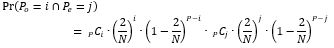
In the terminology used in the derivations so far the term specific passengers has been used. This emphasises the fact that the derivation involves a specified set of i passengers and a specific set of j passengers. But the event will take place if any combination of i passengers in the odd deck are destined for the odd twin floor and if any combination of j passengers in the even deck are destined for its twin even floor. There are a number of different ways in which i passengers can be picked out of a total of P passengers and a number of different ways in which j passengers can be picked out of P passengers in even deck. These are in effect combinations and standard formula for combinations can be used as shown in the equation below.
 (5)
(5)
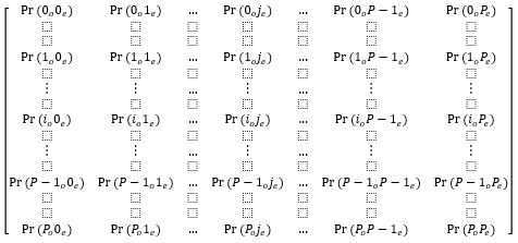
This equation is now used to populate a dedicated matrix as shown below. The row index represents number of passengers heading to the odd floor of the twin pair of floors and the column index represents the number of passengers heading to the even floor of the twin pair of floors. The matrix is a P+1 by P+1 square matrix, as it is important to include the possible case whereby there are no passengers alighting from either deck.
Where: Pr(io je) is the probability that i passengers go to the odd floor and j passengers go to the even floor.
It is worth noting the following points about the different areas of this matrix:
1. The diagonal elements of the matrix represent the cases where the numbers of passengers destined for each of the odd and even floors of the twin are equal. For example, Pr(3o3e) is the probability of three passengers being destined to the odd floor of the twin pair of floors and the three passengers destined to the even floor of the same twin pair of floors.
Pe = Po
In this case, the actual passenger transfer time is the time required for either deck as they are equal (i or j). This is the most efficient case as there is no loss of efficiency in passenger transfer.
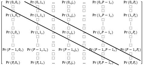
2. The upper triangle of the matrix (i.e., above the diagonal as shown in the figure below) represents the cases where the number of passengers destined for the even twin floor is larger than the number of passengers destined to the odd floor of the twin pair of floors. In other words:
Pe > Po
In this case, the actual passenger transfer time is the time required for the even deck passengers to alight, which is the column index, j. In this case, there is a loss of efficiency in passenger transfer, proportional to the difference between i and j.
3. The lower triangle of the matrix (i.e., below the diagonal) represents the cases where the number of passengers destined to the odd twin floor is larger than the number of passengers destined to the even twin floor. In other words:
Po > Pe
In this case, the actual passenger transfer time is the time required for the odd deck passengers to alight, which is the row index, i. In this case as well, there is a loss of efficiency in passenger transfer, proportional to the difference between i and j.
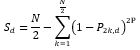
The next step is to find the expected maximum number of passengers alighting. Use will be made of the three areas of the matrix: one equation will be developed for the upper triangle of the matrix, one for the diagonal of the matrix and one for the lower triangle of the matrix.
The expected value of the maximum number of passengers alighting at each stop for the even number of passenger can be found by summing the product of the probability of each number of passengers alighting by their number from the upper triangle of the matrix. The limits of the summations ensure that the number of passengers alighting on the upper (even) deck is larger than the passengers alighting from the lower (odd deck).
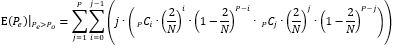 (6)
(6)
The same is repeated for the lower triangle of the matrix as shown in the equation below.
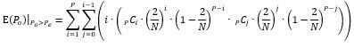 (7)
(7)
Equations (6) and (7) contain two terms: one involves the number of passengers alighting at the even floor and the other the number of passengers alighting at the odd floor.
As for the diagonal terms, there is only one summation and the index runs from 1 to P (the case where both Pe and Po are zero is disallowed, as there would not be a stop in the first place if there are no passengers heading to either floor of the twin).
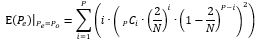 (8)
(8)
Combining all the three cases, it is possible to evaluate the expected value of the maximum number of passengers alighting per twin pair of floors. The expected value is the summation of the three contributions to the expected value in the three cases.
 (9)
(9)
However, there are N/2 twin number of floors, where N is the total number of floors above the main entrance. Thus the expected value of the maximum number of passengers alighting in a round trip is:
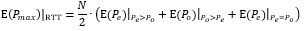 (10)
(10)
Finally, the PTEC is the ratio between the expected value of the maximum number of passengers alighting in each round trip divided by the number of passengers per deck.
 (11)
(11)
The equations derived above for the value of PTEC have been rigorously verified using the Monte Carlo simulation method ([19], [20], [21]) with excellent agreement. More details of numerical examples can be found in [18].
It is expected that the value of the PTEC will improve (i.e., become smaller and more efficient) under destination group control ([22], [23], [24], [25], [26], [27]). This is the current of future research whereby the formula is re-derived under destination group control conditions.
4 The Coefficient Presented by Siikonen
Siikonen derived a coefficient for passenger transfer loading [7]. The derivation will be presented below:
The probable number of stops equals to:
 (12)
(12)
Where P2k,d is the probability of passenger going to 2k-1 or 2k floor.
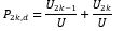 (13)
(13)
The probable number of stops for upper deck only equals to:
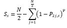 (14)
(14)
Where P2j,s is the probability of passenger going to even floor.
 (15)
(15)
Then, the total passenger transfer time will equal:
 (16)
(16)
This equation assumes that inefficiencies will occur in both alighting and boarding, whereas in this paper the authors have assumed that inefficiency only takes place in alighting and not in boarding. Siikonen also assumes that the population of every twin pair of floor is equal (i.e., the population of the even floor of the twin pair is equal to the population of the odd twin pair) so that the numbers of stop for single deck for odd and even are equal.
5 Numerical Example
In order to gain a numerical appreciation of the range of values of the coefficient (i.e., the PTEC), a numerical example is presented in this section for a realistic range of values for P and N. As discussed earlier in this paper, the coefficient will range from the smallest possible value of 1 (representing full efficiency in passenger alighting from both decks) to the maximum possible value of 2 (representing zero efficiency in passenger alighting from both decks).
Assuming a building with equal floor populations and equal capacity for both decks and an even number of floors above the pair of main entrances, the PTEC was calculated for a range of value of P and N. The results are shown in Table 1.
Table 1: The value of the PTEC for a number of buildings.
| N (number of floors above the main entrance) | ||||||
| P (each deck) | 10 | 12 | 14 | 16 | 18 | 20 |
| 10 | 1.3474 | 1.3848 | 1.4187 | 1.4485 | 1.4763 | 1.5012 |
| 13 | 1.3062 | 1.3411 | 1.3713 | 1.3992 | 1.4243 | 1.4474 |
| 17 | 1.2699 | 1.3001 | 1.3274 | 1.3521 | 1.375 | 1.3958 |
| 20 | 1.2486 | 1.278 | 1.3029 | 1.3262 | 1.3475 | 1.3679 |
| 26 | 1.2186 | 1.2445 | 1.2666 | 1.2875 | 1.3069 | 1.3247 |
As can be seen from the results, the value of the PTEC ranges from around 1.2 up to 1.5. As the number of passengers per deck increases, the efficiency increases (with smaller value of PTEC) as expected. Moreover, as the number of floors above the main entrances increases, the efficiency decreases (with a larger value of PTEC) as expected.
Conclusions
A new parameter has been introduced that measures the efficiency of the passenger transfer time denoted as the PTEC (passenger transfer efficiency coefficient). It represents how efficient the transfer of passenger is when alighting at the destination floors. The PTEC can be used in the calculation of the round trip time whereby it provides an accurate measure of the passenger transfer time. The PTEC has been derived for the case of equal floor populations. The derived equations have been verified using the Monte Carlo Simulation method with excellent agreement. A similar coefficient presented by Siikonen is also studied. A numerical example is given for a number of buildings in order to show the effect of the number of passengers per deck (P) and the number of floors above the pair of main entrances (N) on the value of the coefficient. It is shown that the value of the coefficient increases with the increase in N and decreases with the increase in P.
REFERENCES
- Fortune J. Modern Double Deck Elevator Applications and Theory. Elevator Technology 6 1995; 6: 230-238. Proceedings of the 6th International Conference on Elevator Technologies, Elevcon ’95, Hong Kong March 1995. Published by the International Association of Elevator Engineers.
- CIBSE. CIBSE Guide D: Transportation systems in buildings. Published by the Chartered Institute of Building Services Engineers, Fifth Edition, 2015.
- Barney G C and Al-Sharif L. Elevator Traffic Handbook: Theory and Practice. 2nd Edition. Routledge. 2016.
- Barney G C. Vertical Transportation in Tall Buildings. Elevator World 2003; 51(5): 66-71.
- Binder G. One Hundred and One of the World’s Tallest Buildings. The Images Publishing Group, Victoria, Australia, 2006.
- Al-Sharif L and Seeley C. The effect of the building population and the number of floors on the vertical transportation design of low and medium rise buildings. Building Services Engineering Research and Technology 2010; 31(3): 207-220. doi: 10.1177/0143624410364075. August 2010.
- Siikonen M L. On Traffic Planning Methodology. Elevator Technology 10 2000; 10: 267-274. Proceedings of the 10th International Congress on Elevator Technologies, Berlin Germany May 2000. Published by the International Association of Elevator Engineers.
- Sorsa J, Siikonen M L and Ehtamo H. Optimal control of double-deck elevator group using genetic algorithm. International Transactions in Operational Research 2003; 10: 103-114.
- Tapio Tyni, Jari Yilnen, “Genetic Procedure for Allocating Landing Calls in an Elevator Group”, 25th May 1999, US Patent number: 5907137.
- T. Eguchi, K. Hirasawa, J. Hu, S. Markon, “Elevator group supervisory control systems using genetic network programming”, Congress on Evolutionary Computation, 2004, IEEE, 19th to 23rd June 2004, pp 1661-1667 (volume 2).
- P. Cortes, J. Larraneta, L. Onieva, “Genetic algorithm for controllers in elevator groups: Analysis and simulation during lunch-peak traffic”, Applied Soft Computing, Volume 4, Issue 2, May 2004, Pages 159–174.
- Kavounas G. Elevatoring Analysis with Double Deck Elevators. Elevator World 1989; 37(11): 65-72.
- Peters R D. Lift traffic analysis: General formulae for double deck lifts. Building Services Engineering Research and Technology 1996; 17(4): 209-213.
- Peters R D. General Analysis Double Decker Lift Calculations. Elevator Technology 6 1995; 6: 165-174. Proceedings of the 6 International Conference on Elevator Technologies, Elevcon ’95, Hong Kong March 1995. Published by the International Association of Elevator Engineers.
- Al-Sharif L. Calculating the Elevator Round Trip Time for the Most Basic of Cases (METE II). Lift Report 2014; 40(5): 18-30. Sep/Oct 2014.
- Al-Sharif L, Abu Alqumsan A M and Khaleel R. Derivation of a Universal Elevator Round Trip Time Formula under Incoming Traffic with Stepwise Verification. Building Services Engineering Research and Technology 2014; 35(2): 198–213. doi 0143624413481685.
- Al-Sharif L and Abu Alqumsan A M. Stepwise derivation and verification of a universal elevator round trip time formula for general traffic conditions. Building Services Engineering Research and Technology 2015; 36(3): 311-330. doi: 10.1177/0143624414542111.
- Al-Sharif L, AlOsta E, Abualhomos N and Suhweil Y. Derivation and Verification of the Round Trip Time Equation and Two Performance Coefficients for Double Deck Elevators under Incoming Traffic Conditions. Building Services Engineering Research and Technology 2017; 38(2): 176-196.
- Powell B. The role of computer simulation in the development of a new elevator product. Proceedings of the 1984 Winter Simulation Conference, page 445-450, November 1984, Dallas, TX, USA, published by INFORMS, Catonsville, MD 21228, United States.
- Tam C M and Chan A P C. Determining free elevator parking policy using Monte Carlo simulation. International Journal of Elevator Engineering 1996; 1:24-34.
- Al-Sharif L, Aldahiyat H M and Alkurdi L M. The use of Monte Carlo simulation in evaluating the elevator round trip time under up-peak traffic conditions and conventional group control. Building Services Engineering Research and Technology 2012; 33(3): 319–338. doi:10.1177/0143624411414837.
- Peters R. Understanding the benefits and limitations of destination dispatch. Elevator Technology 16, The International Association of Elevator Engineers, the proceedings of Elevcon 2006, June 2006, Helsinki, Finland, pp 258-269.
- Smith R and Peters R. ETD algorithm with destination dispatch and booster options. Elevator Technology 12 2002; 12: 247-257. The International Association of Elevator Engineers (Brussels, Belgium), proceedings of Elevcon 2002, Milan, Italy, June 2002.
- Joris Schroeder, “Elevatoring calculation, probable stops and reversal floor, “M10” destination halls calls + instant call assignments”, in Elevator Technology 3, Proceedings of Elevcon ’90, International Association of Elevator Engineers, 1990, pp 199-204.
- Sorsa J, Hakonen H and Siikonen M L. Elevator selection with destination control system. Elevator Technology 15 2005; volume 15. The International Association of Elevator Engineers (Brussels, Belgium), proceedings of Elevcon 7th to 9th June 2005, Peking, China.
- Lauener J. Traffic performance of elevators with destination control. Elevator World (Mobile, AL, USA) 2007; 55(9): 86-94.
- Al-Sharif L, Hamdan J, Hussein M, Jaber Z, Malak M, Riyal A, AlShawabkeh M and Tuffaha D. Establishing the Upper Performance Limit of Destination Elevator Group Control Using Idealised Optimal Benchmarks. Building Services Engineering Research and Technology, 2015; 36(5):546-566. September 2015.
BIOGRAPHICAL DETAILS
Lutfi Al-Sharif is currently professor of building transportation systems at the Mechatronics Engineering Department at the University of Jordan, Amman, Jordan. His research interests include elevator traffic analysis and design, elevator and escalator energy modeling and simulation and engineering education.
Enas AlOsta, Noor Abualhomos and Yazan Suhweil all graduated from the department of mechatronics engineering at the University of Jordan, Amman, Jordan in 2017.
Converting the User Requirements into an Elevator Traffic Design: The HARint Space
Lutfi Al-Sharif, Osama F. Abdel Aal,
Mohammad A. Abuzayyad, Ahmad M. Abu Alqumsan
Mechatronics Engineering Department
University of Jordan, Amman 11942, Jordan
This paper was presented at The 3rd Symposium on Lift & Escalator Technology (CIBSE Lifts Group, The University of Northampton and LEIA) (2013). This web version © Peters Research Ltd 2019.
Keywords: Elevator, lift, round trip time, interval, up peak traffic, rule base, Monte Carlo simulation, average travel time, HARint Space, HARint plane.
Abstract. A previous paper introduced the concept of the HARint plane, which is a tool to visualise the optimality of an elevator design. This paper extends the concept of the HARint plane to the HARint space where the complete set of user requirements is used to implement a compliant elevator traffic design.
In the HARint space, the full set of user requirements are considered: the passenger arrival rate (AR%), the target interval (inttar), the average travelling time (ATT) and the average waiting time (AWT).
The HARint space provides an automated methodology in the form a set of clear steps that will allow the designer to convert these four user requirements into an elevator traffic design.
As with the HARint plane method, the target interval is used in combination with the expected arrival rate (AR%) and the building population, U, in order to find an initial assessment the number of passengers expected to board the elevator. The target average travelling time is then used to select a suitable elevator speed. This is then used to calculate the round trip time and then select the optimum number of elevators. An iteration is then carried out to find the actual number of passengers, and hence the elevator capacity. A check is then carried out to ensure that the average waiting time has been met, and if it has not been achieved, then a further iteration is carried out.
While the HARint plane provides the optimum number of elevator cars to achieve the two user requirements, the HARint space provides the optimum number of elevator as well as the optimum rated speed to meet the four user requirements of arrival rate, target interval, average waiting time and average travelling time.
An obvious consequence of the introduction of the average travelling time as a user requirement is that the speed becomes an outcome of the HARint space. The method also triggers a zoning recommendation in cases where the average travelling time cannot be met by varying the speed within reasonable limits.
Introduction
The HARint plane [1] is a methodology that offers the elevator system designer a design methodology to arrive at an elevator design that meets the user requirements of arrival rate (AR%) and target interval (inttar). In addition, it offers the designer a graphical method to visualise the optimality of a design. Following the full set of steps allows the designer to arrive at an elevator design specifying the number of elevators and their car capacity (assuming a preset elevator rated speed).
The HARint plane methodology however is restricted to one rated speed. By covering a number of different speeds at the same time, the HARint space can show at the same time the optimal solution comprising the number of elevators, their rated speed and the car capacity, thus meeting four user requirements.
As with the HARint plane methodology, the HARint space methodology is applicable to incoming traffic conditions.
The HARint Space Methodology
The HARint Space, like the HARint plane, uses two axes to represent the two most important user requirements: the target interval (inttar) and the arrival rate (AR%). The actual interval is represented on the x-axis and the handling capacity (HC%) is represented on the y-axis, corresponding to the two user requirements, respectively. The HARint plane is restricted to one rated speed. The HARint space on the other hand can represent a number of speeds at the same time.
Figure 1 shows an example of the plot of the HARint space. It can be noticed that there are two types of lines on the HARint space: P lines (curved lines shown in black) and L lines (nearly straight lines plotted in colours, green, red and blue). P stands for the number of passengers boarding the car in one round trip. L stands for the number of elevators in the group. These lines intersect at nearly right angles. The P lines pass through all the solutions that have the same number of P passengers. The L lines pass through all the solutions that have the same number of elevators in the group.
However, as different rated speeds are plotted, the P lines do not change with the change of speed, but there are as many L lines for each speed. The L lines have been shown in different colours, where each colour represents a different speed (as shown by the legend).
As with the HARint plane, the optimal solution should meet the two conditions shown in equations (1) and (2) below, with the smallest number of elevators and the lowest rated speed possible (in that order). But in addition it aims to meet the extra two requirements of the target average travelling time and target average waiting time, show in equations (3) and (4) below.
HC% ≥ AR% (1)
intact ≤ inttar (2)
ATTact ≤ ATTtar (3)
AWTact ≤ AWTtar (4)
The P curves and L lines shown in Figure 1 are based on the following numerical example:
Building parameters:
U= 1200 persons (building population)
N= 10 floors (number of floors above main entrance)
df= 4.5 m (floor height)
User requirements
AR%= 12% (arrival rate as a percentage of the building population in 5 minutes)
inttar= 30 s (the target interval)
ATTtar = 60 s (the target average travelling time)
AWTtar = 10 s (the target average waiting time)
Kinematics
v=1.6 m∙s-1, 2.5 m∙s-1, 4.0 m∙s-1 (rated speed)
a= 1 m∙s-2 (rated acceleration)
j= 1 m∙s-3 (rated jerk)
Door timing
tdo= 2 s
tdc = 3 s
Passenger transfer times
tpi=tpo = 1.2 s
An expanded view of the area of interest of the HARint space for this example is shown in Figure 2. It shows three L lines of interest and three P lines of interest. The three L lines are for 4, 5 and 6 elevators in the group. The three P lines are for 10.8, 14.4 and 18.0 passengers in the car. Notes that each L line comprises three coloured lines for the three speeds.
Figure 3 adds the average travelling time to the expanded view that was shown in Figure 2. Each P lines shows the value of the average travelling time corresponding to each speed. For example, the P line with P= 18.0 passengers, corresponds to an average travelling time of 74.4 s, 73.2 s and 73.2 s for the rated speeds of 1.6 m/s, 2.5 m/s and 4.0 m/s respectively. The round trip time can be evaluated using different methods and tools [2, 3, 4, 5, 6, 7]. The average travelling time can either be calculated using a formula for the simple cases [8] or using Monte Carlo simulation for the more complicated cases [9].
Figure 4 shows how the HARint space works in practice. If the P line P=14.4 passengers is used, it leads to a solution shown on point A where the number of elevators in the group is 5, and the rated speed is 2.5 m/s. However, the average travelling time is not met (actual average travelling time is more that the 60 s target). The solution that meets all four user requirements is shown at point B where the actual travelling time is less than 57.5 s and the average waiting time is 3.8 s. This is achieved by using 6 elevators in the group and a speed of 2.5 m/s.
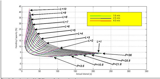
Figure 1: General overview of the HARint space for the example used.
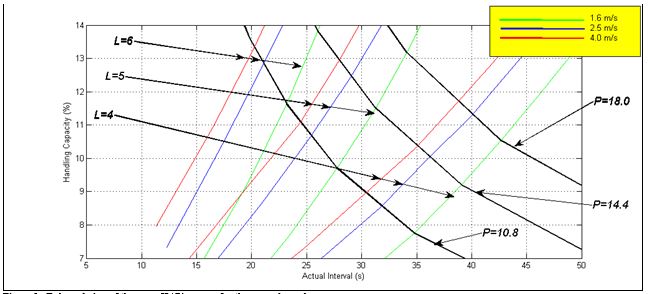
Figure 2: Enlarged view of the same HARint space for the example used.
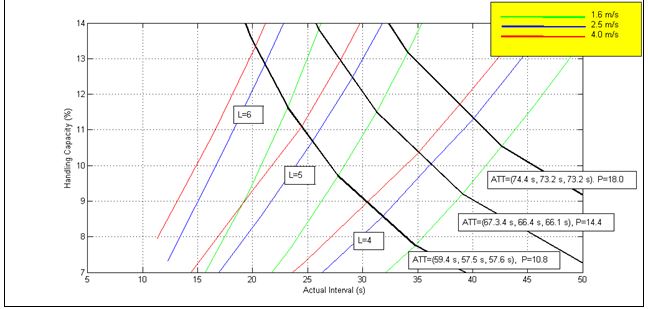
Figure 3: A view that shows that the constant P lines are also constant ATT lines.
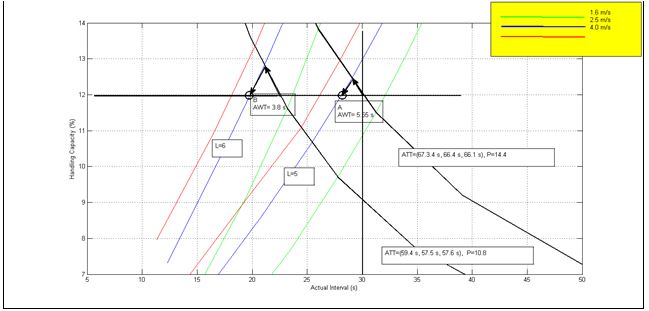
Figure 4: Two solutions A and B, one that meets the ATT requirement and one that does not.
Conclusions
The HARint space has been presented as a methodology that uses four user requirements in order to develop a compliant elevator traffic design. It relies on graphical methods to visualise the final solution.
The four user requirements are: the passenger arrival rate (AR%), the target interval (inttar), the target average travelling time (ATTtar) and the target average waiting time (AWTtar).
A comparison is shown below in table format between the HARint plane method and the HARint space method. The HARint space offers the advantage that it provides the optimum rated speed and meets all the four user requirements instead of just two requirements as is the case in the HARint plane.
| Category | The HARint Plane | The HARint Space |
| User requirements |
|
|
| Optimal outputs |
|
|
| Byproduct output |
|
|
| Triggers |
|
REFERENCES
- Lutfi Al-Sharif, Ahmad M. Abu Alqumsan, Osama F. Abdel Aal, “Automated optimal design methodology of elevator systems using rules and graphical methods (the HARint plane)”, Building Services Engineering Research & Technology, August 2013 vol. 34 no. 3, pp 275-293, doi: 10.1177/0143624412441615.
- CIBSE, “CIBSE Guide D: Transportation systems in buildings”, published by the Chartered Institute of Building Services Engineers, Fourth Edition, 2010.
- G. C. Barney, “Elevator Traffic Handbook: Theory and Practice”, Spon Press, London and New York, ISBN 0-415-27476-1, 2003.
- Richard Peters, “Lift traffic analysis: Formulae for the general case”, Building Services Engineering Research & Technology, 11(2), 1990, pp 65-67.
- Lutfi Al-Sharif, Ahmad M. Abu Alqumsan, Rasha Khaleel, “Derivation of a Universal Elevator Round Trip Time Formula under Incoming Traffic”, Building Services Engineering Research and Technology 0143624413481685, first published on-line June 13th, 2013 as doi:10.1177/0143624413481685.
- Lutfi Al-Sharif, Hussam Dahyat, Laith Al-Kurdi, “ The use of Monte Carlo Simulation in the calculation of the elevator round trip time under up-peak conditions”, Building Services Engineering Research and Technology, volume 33, issue 3 (2012) pp. 319–338, doi:10.1177/0143624411414837.
- Lutfi Al-Sharif, Ahmad Hammoudeh, “Evaluating the Elevator Round Trip Time for Multiple Entrances and Incoming Traffic Conditions using Markov Chain Monte Carlo”, International Journal of Industrial and Systems Engineering (IJISE), Inderscience Publishers, accepted for publication on 4th June 2013.
- http://www.inderscience.com/info/ingeneral/forthcoming.php?jcode=ijise
- So A.T.P. and Suen W.S.M., "New formula for estimating average travel time", Elevatori, Vol. 31, No. 4, 2002, pp. 66-70.
- Lutfi Al-Sharif, Osama F. Abdel Aal, Ahmad M. Abu Alqumsan, “The use of Monte Carlo simulation to evaluate the passenger average travelling time under up-peak traffic conditions”, Chartered Institute of Building Services Engineers, Symposium on Lift and Escalator Technologies, 29th September 2011, University of Northampton, United Kingdom (www.liftsymposium.org/index.php/previous-events).
The use of Monte Carlo simulation to evaluate the passenger average travelling time under up-peak traffic conditions
Lutfi Al-Sharif, Osama F. Abdel Aal, Ahmad M. Abu Alqumsan
Mechatronics Engineering Department
University of Jordan, Amman 11942, Jordan
This paper was presented at the 1st Symposium of Lift and Escalator Technologies (CIBSE Lifts Group and The University of Northampton) (2011). This web version © Peters Research Ltd 2019
Abstract
Monte Carlo simulation is a powerful tool used in calculating the value of a variable that is dependent on a number of random input variables. For this reason, it can be successfully used when calculating the round trip time of an elevator, where some of the inputs are random and follow preset probability distribution functions. The most obvious random inputs are the number of passengers boarding the car in one round trip, their origins (in the case of multiple entrances) and their destinations.
Monte Carlo simulation has been used to evaluate the elevator round trip time under up-peak traffic conditions. Its main advantage over analytical formula based methods is that it can deal with all special conditions in a building without the need for evaluating new special formulae. A combination of all of the following special conditions can be dealt with: Unequal floor population, unequal floor heights, multiple entrances and top speed not attained in one floor jump. Moreover, this can be done without loss of accuracy, by setting the number of runs to the appropriate value.
This paper extends the previous work on Monte Carlo simulation in relation to two aspects: the passenger arrival process model and the passenger average travelling time.
The software is developed using MATLAB. The results for the average travelling time are compared to analytical formulae (such as that by So. et al., 2002). The results showing the effect of the Poisson arrival process on the value of the elevator round trip time are also analysed.
The advantage of the method over analytical methods is again demonstrated by showing how it can deal with the combination of all the special conditions without the loss of accuracy (five conditions if the passenger arrival model is added as Poisson).
The issues of convergence, accuracy and running time are discussed in relation to the practicality of the method.
Keywords: Monte Carlo simulation, elevator, lift, round trip time, interval, up peak traffic, average waiting time, average travelling time, multiple entrances, highest reversal floor, probable number of stops.
Nomenclature
a is the top acceleration in m/s2
AR% is the passenger arrivals expressed as a percentage of the building population in the busiest five minutes
att is the average travelling time in s
awt is the average waiting time in s
CC is the car carrying capacity in persons
df is the height of one floor in m
df(i) is the floor height for floor i
df eff is the effective floor height used in the case of unequal floor heights in m
E(dtotal) is the expected value of the distance travelled in the up direction in m
dG is the height of the ground in m where more than the typical floor height
E(df) is the expected value of the floor heights (effective floor height)
H is the highest reversal floor (where floors are numbered 0, 1, 2….N
HC% is the handling capacity expressed as a percentage of the building population in five minutes
int is the interval at the main terminal in s
j is the top rated speed in m/s3
L is the number of the elevators in the group
N is the number of floors above the main terminal
P is the number of passengers boarding the car from the main terminal (does not need to be an integer)
S is the probable number of stops is the round trip time in s
tao is the door advance opening time in s (where the door starts opening before the car comes to a complete standstill)
tdc is the door closing time in s
tdo is the door opening time in s
tf is the time taken to complete a one floor journey in s
tpi is the passenger boarding time in s
tpo is the passenger alighting time in s
tpB is the component of the travelling time that the passenger spends boarding and alighting from the elevator car in s
tpW is the component of the travelling time that the passenger spends waiting for other passengers to board and alight from the elevator car in s
tpH is the component of the travelling time that the passenger spends travelling in the up direction at rated speed in s
tpS is the component of the travelling time that the passenger spends stopping when travelling in the up direction in s (accelerating, decelerating times, door opening and closing times)
ts is the time delay caused by a stop in s
tsd is the motor start delay in s
tv is the time required to traverse one floor when travelling at rated speed in s
U is the total building population
Ui is the building population on the ith floor
v is the top rated speed in m/s
1. Introduction
Monte Carlo simulation is a powerful method that can be used to evaluate the output value for problems that have a number of random inputs, whereby the probability density functions of the input random variables are known. By generating instances of the random input variable in the form of scenarios, and running a large number of scenarios, the expected value of the output of interest can be found by taking the average value of all the scenarios. Scenarios in this paper will be referred to as trials.
Monte Carlo simulation has been effectively used to evaluate the round trip time under up peak traffic conditions [1], in finding an optimum parking policy [2] as well as generating passengers for the purposes of simulating [3]. It offers an advantage over conventional equation based methods where special conditions exists, such as unequal floor heights, unequal floor populations, top speed not attained in one journey and multiple entrances.
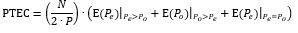
This paper extends the application of the method to the calculation of the passenger average travelling time. In order to verify the results of the method, an equation is developed to calculate the average travelling time under up peak traffic conditions assuming top speed is attained in one floor journey, single entrance and equal floor heights. The Monte Carlo simulation results for the average travelling time are then compared to the equation developed in [4]. The equation is then extended in order to cover the case of unequal floor heights.
Analytical methods for elevator traffic analysis have been extensively covered in [5], [6], [7] and [8]. The Poisson passenger arrival model has been extensively covered in [9], [10], [11] and [12]. The case of the top speed not attained in one floor journey is addressed in [13]. The case of multiple entrances has been addressed in [14]. Discrete time-slice Simulation based methods have been developed in [15].
In order to ensure consistency and clarity of the interpretation of the results, the following definitions will be used throughout this paper for the average waiting time (awt) and the average travelling time (att):
awt: The average waiting time will be defined as the period from passenger arrival in the lobby until the passenger starts to board the car. Thus, based on this definition, the average waiting time does not include the passenger boarding time.
att: The average travelling time will be defined as the period from the time the passenger starts to board the car until the passenger has left the car at the destination floor. Thus, based on this definition, the average travelling time does include the passenger boarding time. It also includes the passenger alighting time at the destination.
The equation for the average travelling time is derived in section 2. Verification of this equation using the Monte Carlo simulation method is carried out in section 3. The equation is then further adjusted for the case of unequal floor heights in section 4. The effect of the Poisson passenger arrival model is analysed in section 5. A practical elevator system design example is given in section 6. A number of notes on convergence are presented in section 7. Conclusions and further work is presented in sections 8 and 9 respectively.
2. Dervation of the equation for the average travelling time
An equation for the average travelling time has been developed in [4]. The equation is derived in the section using a different approach and in accordance with definition presented earlier.
The approach that will be followed in deriving the average travelling time is to find the expression for each component of the minimum possible time and maximum possible time and the use the average of both.
The average travelling time includes four components:
- The boarding and alighting time for the passenger himself/herself.
- The time the passenger spends waiting for other passengers to board and alight.
- The time the passenger spends during the elevator stoppage time (where stoppage time includes acceleration and deceleration time as well as door opening and closing times).
- The time that the passenger spends in the elevator car travelling at top speed.
The first component, which is the boarding and alighting time of the passenger, is easy to evaluate:
![]() (1)
(1)
In order to calculate the second component, it is assumed that on average the passenger will have the remaining P −1 passengers ahead of him/her and the other half behind him/her. Thus he/she will have to wait for  passenger to board the elevator after he/she has boarded; and will have to wait for passenger to alight before he/she could alight.
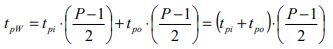 (2)
(2)
As for the time spent during elevator stops, it is worth noting that all passengers will at least have to wait for the first stop (rational passenger boarding at the ground cannot alight at the ground and must at least wait for the first stop). Thus all passengers as a minimum must wait for ts caused by the first stop. As a maximum, a passenger might have to wait for all the S stops above, S⋅ts. None of the passengers will wait the last stop (door closing at the highest floor, acceleration and deceleration during the express back journey and doors opening at the main entrance) and hence the wait is for S stops rather than S+1 stops. Taking the average of both values above, gives the average time each passenger waits during elevator stops travelling in the up direction:
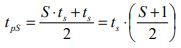 (3)
(3)
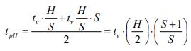
On average each stop will traverse a distance of  floors. All passengers will have to wait for that distance to be traversed at stop speed at least, as any rational passenger cannot board at the main terminal and leave at the main terminal. As a maximum, some passengers will have to wait for the whole H floors to be traversed. The minimum time will be tv. ,while the maximum time will be
  Taking the average of both times give an expression for the time spent during travelling at top speed in the up direction.
 (4)
(4)
Adding all the four terms provides an expression for the average travelling time:
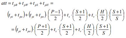 (5)
(5)
Rearranging and assuming that tpi = tpo = tp, gives the important final result for the average travelling time:
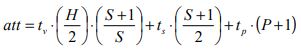 (6)
(6)
A similar expression for the average travelling time has been derived by So () using a different method and is shown below:
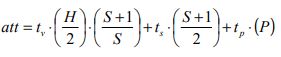 (7)
(7)
It is worth noting that the expression in equation (6) differs from the one in equation (7) in that it includes an extra tp where this accounts for the fact that this definition of waiting time includes passenger boarding time, while equation (7) excluded passenger boarding time.
It is also worth noting that equations (6) and (7) implicitly make the following assumptions:
- Top speed is attained on one floor journey.
- Incoming up peak traffic only.
- Equal floor heights.
- Single entrance.
The equation of the round trip time depends on the values of S (probable number of stops), H (the highest reversal floor) and P (the number of passengers in the car) as shown in equation (16).
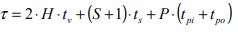 (8)
(8)
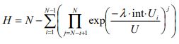
The highest reversal floor is a function of the number of passengers:
 (9)
(9)
The probable number of stops is also a function of the number of passengers:
 (10)
(10)
The number of passengers in the elevator car is equal to the product of the passenger arrival rate and the actual interval:
 (11)
(11)
But the interval is in fact a function of the round trip time as shown in equation (20) below:
 (12)
(12)
Combining equations (19) and (20) gives the following result that shows that the number of passengers is a function of the round trip:
 (13)
(13)
As can be concluded from the two equations ((8) and (13)) the round trip time is a function of the number of passengers, but the number of passengers is a function of the round trip time. Thus the equation for the round trip time shown in (8) is an implicit equation of the round trip time that can be only solved by the use of an iterative approach (or other mathematical methods such as conformal mapping [11]). This has been addressed as part of a comprehensive design methodology [17].
When amending the equations for H and S to address the Poisson passenger arrival model, the term that represents the probability of a passenger not travelling to the ith floor can be amended as shown below.
The probability of a passenger will not travel to floor i assuming equal floor populations for constant and Poisson arrival modes is shown below (using equation (11)):
| Constant passenger arrival model |
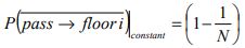 |
(14) |
| Poisson passenger arrival model |
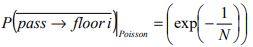 |
(15) |
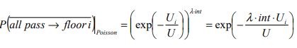
The probability that all the passengers will not go to a floor i is (assuming equal floor populations) for both constant and Poisson arrival models is shown below:
| Constant passenger arrival model with equal floor populations |
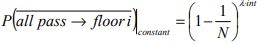 |
(16) |
| Poisson passenger arrival model with equal floor populations |
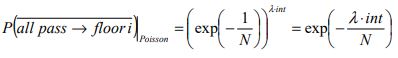 |
(17) |
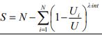
And this can be further developed for the case of unequal floor populations as shown below:
| Constant passenger arrival model with equal floor populations |
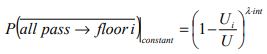 |
(18) |
| Poisson passenger arrival model with equal floor populations |
 |
(19) |
The probability of all passengers not going to a floor i is equivalent to the probability of the elevator not stopping at floor i. These expressions are used in deriving the values of H and S as shown in equations (20) to (27).
The equation for calculating the average travelling time (8) can cope with a number of special conditions such as unequal floor heights and Poisson arrival model by using the calculated for the probable number of stops and the highest reversal floor in accordance with equations (20) to (27).
| Constant passenger arrival model | Poisson passenger arrival model | |||
| Equal floor populations |
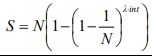 |
(20) | 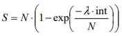 |
(21) |
|
Unequal floor |
 |
(22) |  |
(23) |
| Constant passenger arrival model | Poisson passenger arrival model | |||
|
Equal floor |
 |
(24) |  |
(25) |
|
Unequal |
 |
(26) |  |
(27) |
3. Verification
The derivation of the equation for the average travelling time has been necessary in order to verify the use of the Monte Carlo simulation. A repeat of the calculations carried out in [4] has been carried out with the results shown in Table 1. The results show excellent agreement with the calculation results.
Table 1: Verification results for the average travelling time comparing calculation and Monte Carlo simulation.
| N | P | Analytical Equation, assuming constant arrival process (7) |
Monte Carlo Simulation (assuming constant arrival process) |
| 10 | 6.4 | 48.19 | 48.18 |
| 10 | 16.8 | 74.46 | 74.40 |
| 13 | 6.4 | 53.65 | 53.67 |
| 13 | 16.8 | 84.00 | 84.00 |
| 16 | 10.4 | 73.27 | 73.27 |
| 16 | 20.8 | 101.97 | 101.97 |
| 20 | 10.4 | 80.70 | 80.72 |
| 20 | 20.8 | 112.85 | 112.85 |
| 23 | 12.8 | 94.74 | 94.65 |
| 23 | 26.4 | 135.00 | 135.03 |
However, the strength of the Monte Carlo simulation method becomes clear when the special conditions exist (such as top speed not attained or multiple entrances), where the calculation method fails to deal with. This will be illustrated later in this paper.
4. Case of unequal floor heights
In the case where the floor heights are unequal, this will have an effect on the calculation of the round trip time equation. The equation for the round trip time or average travelling time can be amended as follows in order to account for this case as follows.
The effect of the unequal floor heights can be taken into consideration by assuming an effective floor height df eff that can be inserted into the original round trip time equation. The effective floor height df eff is the expected value of the floor height. The effective floor height is the weighted average of all the floor heights multiplied by the probability of the elevator passing through that floor. In order for the elevator to pass through a floor it should travel to any of the floors above that floor. Thus it is necessary to find the probability of the elevator travelling above a certain floor, i.
The probability of the elevator not stopping at a certain floor, assuming equal floor populations is the probability that passenger j will stop at a floor i (assuming equal floor populationand a constant passenger arrival model):
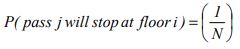 (27)
(27)
Thus the probability that passenger j will not stop at a floor i is:
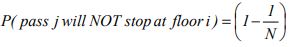 (28)
(28)
But the car contains P passengers. So the probability that none of them will stop at floor i is the product of all of their respective probabilities:
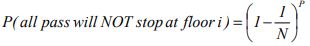 (29)
(29)
The probability that the lift will not travel any higher than a floor i is the probability that it will not stop on floor i+1 or i+2 or i+3 all the way to floor N. This is expressed as the product of these individual conditional probabilities:
P (lift will not travel above floor i)=
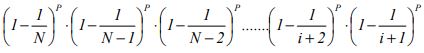 (30)
(30)
This can be re-written as:
P (lift will not travel above floor i)=
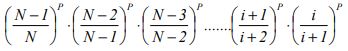 (31)
(31)
Putting all terms inside the same bracket gives:
P(lift will not travel above floor i)=
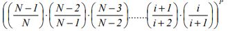 (32)
(32)
This simplifies to:
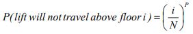 (33)
(33)
Thus the probability that the lift will travel above the floor i is:
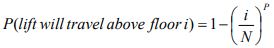 (34)
(34)
Thus the expected value of the travel distance can be calculated as the weighted average of the various floor heights as follows:
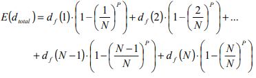 (35)
(35)
The last term above reduces to zero (as it is impossible for the elevator to pass through floor N). The expected floor height is obtained by dividing the expected total travel distance by the highest reversal floor, H. So the equation for the effective floor height can be expressed as shown below (assuming equal floor populations and a constant passenger arrival model):
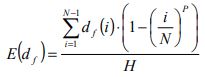 (36)
(36)
The same procedure can be used to develop the equation for the case of unequal populations and Poisson passenger arrival model.
Taking an example to illustrate the difference in the effective floor height, a building with 20 floors above ground is analysed. The floor heights are shown below in Table 2. It will be assumed that the floor populations are equal and that the passenger arrival process is constant (rather than Poisson). It will be also assumed that the number of passenger, P, is 13.
Table 2: The floor heights for a building with 20 floors above ground.
| Floor # | i | df(i) (m) |
| L20 | 21 | 3.2 |
| L19 | 20 | 3.2 |
| L18 | 19 | 3.2 |
| L17 | 18 | 4.2 |
| L16 | 17 | 4.2 |
| L15 | 16 | 4.2 |
| L14 | 15 | 4.2 |
| L13 | 14 | 4.2 |
| L12 | 13 | 4.2 |
| L11 | 12 | 4.2 |
| L10 | 11 | 4.2 |
| L9 | 10 | 4.2 |
| L8 | 9 | 4.2 |
| L7 | 8 | 4.2 |
| L6 | 7 | 4.2 |
| L5 | 6 | 4.2 |
| L4 | 5 | 4.2 |
| L3 | 4 | 6 |
| L2 | 3 | 6 |
| L1 | 2 | 6 |
| G | 1 | 8 |
Applying equation (24) to evaluate the highest reversal floor gives a value for H of: 18.95 (assuming floors numbers run from 1 to 21). Then applying equation (36) to evaluate the effective floor height gives a value of 4.62 m. This can be compared to the average floor height of all floors, which is 4.50 m. A difference of 0.12 m exists per floor.
The average passenger travelling time can be calculated in order to assess the effect of unequal floor heights, using equation (7). Using the parameters shown below, whereby the rated speed is attained in one floor journey, and there is only a single entrance and a constant passenger arrival model is assumed.
tdo = 2 s
tdc = 3 s
tsd = 0.5 s
tao = 0 s
tpi = 1.2 s
tpo = 1.2 s
v = 1.6 m/s
a = 1.0 m/s2
j = 1.0 m/s3
The calculation and Monte Carlo simulation results for both round trip time and the average travelling time are shown in Table 3 below.
Table 3: Calculation and Monte Carlo simulation results for the round trip time and the average travelling time (all results in seconds).
| Floor height used | Round trip time | Average travelling time | ||
| Calculation | Monte Carlo simulation |
Calculation | Monte Carlo simulation |
|
| Average of all floor heights (4.5 m) |
225.11 | 225.10 | 89.76 s | 89.83 |
| Effective floor height 4.62 m using equation () |
227.96 | 227.96 | 90.55 s | 90.55 |
Using the effective floor height results in a difference of around 3 seconds for the round trip time and a difference of around 1 second for the average travelling time. Moreover, the Monte Carlo simulator is giving identical results to the calculation method of the amended equation.
5. The effect of the Poisson Passenger Arrival Model
Further investigation is carried out in this section of the effect of the passenger arrival model on the round trip time and the average travelling time. Table 4 shows the average travelling time and the round trip time for a number of buildings using for both the constant passenger arrival model and the Poisson arrival model. It can be seen that the assumption of a Poisson arrival model results in a small reduction of the values of the round trip time and the average travelling time.
Table 4: Round trip time and average travelling time for the two passenger arrival models.
| N | P | Analytical Equation, assuming constant arrival process (equation (7)) |
Monte Carlo Simulation (assuming constant arrival process) |
Monte Carlo Simulation (assuming Poisson arrival process) |
||
| att | att | τ | att | τ | ||
| 10 | 6.4 | 48.19 | 48.18 | 114.26 | 47.37 | 111.72 |
| 10 | 16.8 | 74.46 | 74.40 | 170.82 | 73.90 | 169.49 |
| 13 | 6.4 | 53.65 | 53.67 | 131.27 | 53.08 | 128.83 |
| 13 | 16.8 | 84.00 | 84.00 | 197.40 | 83.36 | 195.75 |
| 16 | 10.4 | 73.27 | 73.27 | 180.98 | 72.60 | 178.80 |
| 16 | 20.8 | 101.97 | 101.97 | 241.80 | 101.25 | 240.21 |
In general, as the number of passengers changes, the Poisson arrival model results in a smaller value of the round trip time and the average travelling time, as shown in Figure 1 and Figure 2 respectively.
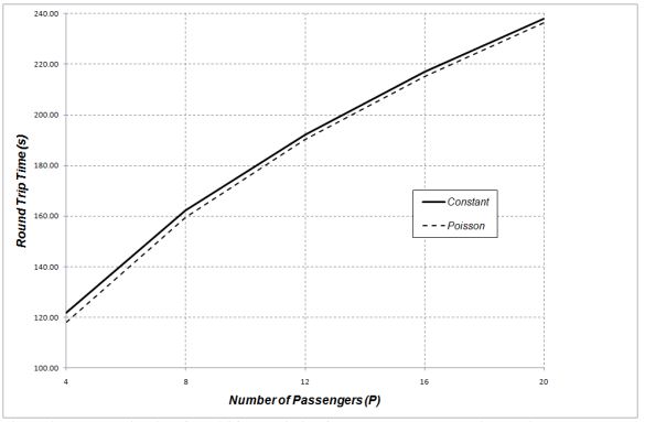
Figure 1: Round Trip Time for a 16 floor building for both constant and Poison arrival passenger models.
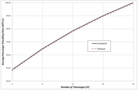
Figure 2: Average travelling time for a16 floor building under constant and Poisson passenger arrival models.
6. Practical example
In order to illustrate the use of the Monte Carlo Simulation method in the elevator traffic design, the following practical example is presented. The example is shown in order to illustrate the use of the method for the combination of all of the following special cases:
a. Constant passenger arrival model.
b. Unequal floor populations.
c. Unequal floor heights.
d. Top speed not attained in one floor journey.
e. Multiple entrances.
An office building has an arrival rate (AR%) of 12%. It is desired to design the elevator system such that a target interval of 30 seconds is achieved. The automated design method developed in [17] is used for the design and the Monte Carlo simulation is used to calculate the round trip time as shown in [1].
The following parameters are used:
tdo = 2 s
tdc = 3 s
tsd = 0.5 s
tao = 0 s
tpi = 1.2 s
tpo = 1.2 s
v = 4.0 m/s (top speed will not be attained in one floor journey [16])
a = 1.0 m/s2
j = 1.0 m/s3
Table 5: The floor heights, populations and arrival rates for a building with 20 floors above ground.
| Floor # | df(i) (m) | Entrance arrival percentage |
Population |
| L20 | 4 | - | 30 |
| L19 | 4 | - | 38 |
| L18 | 4 | - | 38 |
| L17 | 4 | - | 38 |
| L16 | 4 | - | 38 |
| L15 | 4 | - | 38 |
| L14 | 4 | - | 38 |
| L13 | 4 | - | 38 |
| L12 | 4 | - | 38 |
| L11 | 4 | - | 38 |
| L10 | 4 | - | 38 |
| L9 | 4 | - | 38 |
| L8 | 4 | - | 38 |
| L7 | 4 | - | 38 |
| L6 | 4 | - | 38 |
| L5 | 4 | - | 38 |
| L4 | 4 | - | 100 |
| L3 | 6 | - | 100 |
| L2 | 6 | - | 100 |
| L1 | 6 | - | 100 |
| G | 8 | 70% | - |
| B1 | 3.2 | 10% | - |
| B2 | 3.2 | 10% | - |
| B3 | 3.2 | 10% | - |
The resultant design is shown below:
- Constant passenger arrival model
- Round trip time: 177.72 s
- Average travelling time: 71.73 s
- Number of elevators: 7
- Target interval: 30 s
- Actual Interval: 25.39 s
- Actual passenger P: 10.15 passengers
- Car capacity: 13 passengers 1000 kg
- Car loading: 78%
7. Notes on Convergence of the Monte Carlo Simulator
In this section, some analysis is carried out on the convergence of the final result from the Monte Carlo simulator as used to calculate the round trip time and the passenger average travelling time.
In order to achieve better accuracy, the number of trials can be selected. The round trip time results for a sample building are shown in Table 6. For each number of trials, the analysis is carried out 10 times.
Table 6: Effect of the number of trials on the calculation of the round trip time using the Monte Carlo Simulator.
| Number of Trials | ||||||
| Readings for the round trip time (s) |
10 | 100 | 1000 | 10000 | 100000 | 1000000 |
| 150 | 154.7813 | 153.8286 | 154.1935 | 154.1368 | 154.1514 | |
| 153.87 | 153.8205 | 154.3263 | 154.1499 | 154.205 | 154.1547 | |
| 152.745 | 152.9183 | 153.6842 | 153.8559 | 154.1622 | 154.1546 | |
| 155.7375 | 152.6933 | 153.7789 | 153.9662 | 154.1579 | 154.1587 | |
| 154.6125 | 153.4088 | 154.1551 | 154.0913 | 154.1548 | 154.1553 | |
| 156.3 | 155.4473 | 153.8216 | 154.2747 | 154.1166 | 154.1585 | |
| 156.5475 | 154.0455 | 154.0831 | 154.1364 | 154.1485 | 154.1510 | |
| 162.2175 | 153.3323 | 154.5007 | 154.1614 | 154.2053 | 154.1533 | |
| 156.5475 | 153.708 | 154.4249 | 154.1944 | 154.1861 | 154.1614 | |
| 147.75 | 155.049 | 154.2289 | 154.1461 | 154.1513 | 154.1557 | |
The results of all the Monte Carlo Simulations are plotted as a scatter diagram in Figure 3 in order to visually convey the relationship between the accuracy of the method against the number of trials. The effect on accuracy of the final answer against the number of trials is plotted in Figure 4. Based on the results in the figure, 100 000 trials are required for accuracies better than ±0.1%.
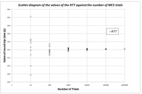
Figure 3: Convergence of the value of the round trip as the number of trials is increased.
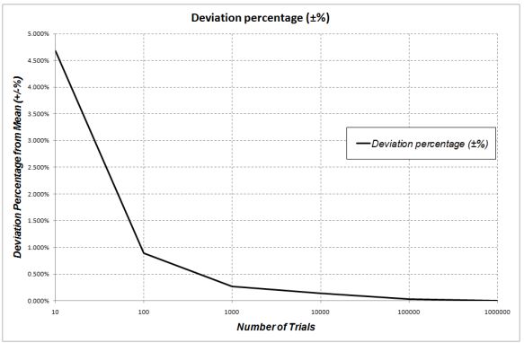
Figure 4: Deviation percentage of the RTT from the mean against the number of trials.
For the example above, an analysis is shown of the running time for the increased number of trials and the resultant accuracy, as shown in below. This provides a guide to the designer in terms of trading off accuracy with running time.
It is worth noting that these running times are based on the running of MATLAB code. Use of other tools, such as C++ for example, would provide much faster software, significantly reducing the running time.
Table 7: Accuracy of the results for different number of trials and the required running time for the Monte Carlo Simulation for the example used.
| Number of iterations | Percentage deviation from the mean |
Running time (s) (for the example of 10 floors above ground, 13 passengers) |
| 10 | ±4.678% | <1 |
| 100 | ±0.895% | <1 |
| 1000 | ±0.265% | <1 |
| 10000 | ±0.136% | <1 |
| 100000 | ±0.029% | 7 |
| 1000000 | ±0.003% | 70 |
8. Conclusions
Monte Carlo simulation has been used to calculate the average passenger travelling time in an elevator system under up peak traffic conditions. The results of the Monte Carlo simulation have been verified for the simplest cases using an analytical formula for the average travelling time that has been derived. This verification showed good agreement.
The analytical equation was further developed to deal with the case of unequal floor heights, and further verification was carried out with good agreement. The analytical equations for the average travelling time can be applied to the cases of unequal floor populations and Poisson passenger arrival model.
The strength of the Monte Carlo simulation comes to the fore when the combination of all the five special conditions exists in a building: unequal floor heights; unequal floor populations; multiple entrances; Poisson arrival model and top speed not attained. A practical design example is given to show how the method can be used to calculate the round trip time and the average travelling time.
Commentary is given on the rate of convergence of the method, and the effect of the number of trials on the accuracy of the result. A guide is provided to the designer as to the trade-off between the number of trials, accuracy of the method and the running time.
REFERENCES
- Lutfi Al-Sharif, Husam M. Aldahiyat, Laith M. Alkurdi, “The Use of Monte Carlo Simulation in Evaluating the Elevator Round Trip Time under Up-peak Traffic Conditions”, accepted for publication in Building Services Engineering Research & Technology, 2/6/2011.
- C. M. Tam, Albert P. C. Chan, “Determining free elevator parking policy using Monte Carlo simulation”, International Journal of Elevator Engineering, Volume 1, 1996, page 24 to 34.
- Bruce A. Powell, “The role of computer simulation in the development of a new elevator product”, Proceedings of the 1984 Winter Simulation Conference, page 445-450, 1984.
- So A.T.P. and Suen W.S.M., "New formula for estimating average travel time", Elevatori, Vol. 31, No. 4, 2002, pp. 66-70.
- CIBSE, “CIBSE Guide D: Transportation systems in buildings”, published by the Chartered Institute of Building Services Engineers, Third Edition, 2005.
- G.C. Barney, “Elevator Traffic Handbook: Theory and Practice”, Taylor & Francis, 2002.
- R. D. Peters, “Lift Traffic Analysis: Formulae for the general case”, Building Services Engineering Research and Technology, Volume 11 No 2 (1990)
- Richard D. Peters, “The theory and practice of general analysis lift calculations”, Proceedings of the 4th International Conference on Elevator Technologies (Elevcon ’92), Amsterdam, May 1992.
- N. A. Alexandris, G. C. Barney, C. J. Harris, “Multi-car lift system analysis and design”, Applied Mathematical Modelling, 1979, Volume 3 August.
- N. A. Alexandris, G. C. Barney, C. J. Harris, “Derivation of the mean highest reversal floor and expected number of stops in lift systems”, Applied Mathematical Modelling, Volume 3, August 1979.
- N. A. Alexandris, C. J. Harris, G. C. Barney, “Evaluation of the handling capacity of multicar lift systems”, Applied Mathematical Modelling, 1981, Volume 5, February.
- N. A. Alexandris, “Mean highest reversal floor and expected number of stops in lift-stairs service systems of multi-level buildings”, Applied Mathematical Modelling, Volume 10, April 1986.
- N.R. Roschier, M.J., Kaakinen, "New formulae for elevator round trip time calculations", Elevator World supplement, 1978.
- Lutfi Al-Sharif, , “The effect of multiple entrances on the elevator round trip time under uppeak traffic”, Mathematical and Computer Modelling, Volume 52, Issues 3-4, August 2010, Pages 545-555.
- Richard David Peters, “Vertical Transportation Planning in Buildings”, Ph.D. Thesis, Brunel University, Department of Electrical Engineering, February 1998.
- Richard D. Peters, “Ideal Lift Kinematics”, Elevator Technology 6, IAEE Publications, 1995.
- Lutfi Al-Sharif, Ahmad M. Abu Alqumsan, Osama F. Abdel Aal, “Automated Optimal Design Methodology of Elevator Systems using Rules and Graphical Methods (the HARint plane)”, under review, Building Services Engineering Research & Technology, 17/6/2011.
The HARint plane: A Graphical Method for Visualising the Optimality of an Elevator System Design Option
Lutfi Al-Sharif, Ahmad M. Abu Alqumsan, Osama F. Abdel Aal
Mechatronics Engineering Department
University of Jordan, Amman 11942, Jordan
This paper was presented at The 2nd Symposium on Lift & Escalator Technology (CIBSE Lifts Group, The University of Northampton and LEIA) (2012). This web version © Peters Research Ltd 2019.
Keywords: Elevator, lift, round trip time, interval, up peak traffic, rule base, Monte Carlo simulation, average travel time, HARint plane.
Abstract: This paper presents a graphical methodology of visualizing the optimality of an elevator design solution. It introduces a new plane called the HARint plane, each point on which represents a solution to the elevator design problem.
By visually inspecting the plane and examining the intersection of various curves on the plane, the designer can understand how far the offered solution is from the optimal solution and also whether the offered design is wasteful.
The HARint plane comprises the quality of service, represented by the actual interval and the quantity of service, represented by the handling capacity. These are compared with the client/site requirements in terms of the target interval and the arrival rate. A number of curves can then be plotted on the plane based on the possible number of elevators and the car loading in passengers.
In drawing the curves on the plane, the round trip time has to be known. The round trip time can either be calculated analytically or by the use of Monte Carlo simulation. However, the calculation of the round trip time is only part of the design methodology. This paper does not discuss the round trip time calculation methodology as this has been addressed in detail elsewhere.
The optimality of the design is assessed by a clear step by step methodology that uses the user requirements to select an optimal design.
1. Introduction
The round trip time is the time needed by the elevator to complete a full journey in the building, taking passengers from the main entrance(s) and delivering them to their destinations and then expressing back to the main entrance, under up peak (incoming) traffic conditions.
This paper presents a step-by-step automated method for elevator design under specific arrival conditions, assuming that a method exists for calculating the round trip time. It uses a combination of rules and graphical methods to arrive at an optimal solution. A graphical tool, called the HARint plane, is presented as a means to visualise the solution.
The fact that the methodology is fully automated makes it very attractive for implementation as a software package. It has also been used for teaching elevator traffic analysis to final year undergraduate mechatronics engineering students.
Full details on the use of the method in optimising the number of elevators as well as the speed and capacity can be found in [1].
2. The problem with conventional design methods
It will be assumed that the designer starts with the knowledge of the following parameters that are given either by the architect or the building owner or that can be inferred from the type of occupancy (e.g., office, residential…etc.). These represent the user requirements.
a) The total building population, U. If this is not given directly, it can be calculated from either net floor area of the gross floor area.
b) The expected arrival rate, AR%. This is the percentage of the building population arriving in the building during the busiest five minutes. This value depends on the type of building occupancy.
c) The target interval inttar.
A sufficient design meets the following two conditions:
HC% ≥ AR% (1)
intact ≤ inttar (2)
…where:
AR% is the arrival rate expressed as a percentage of the building population in five minutes
HC% is the handling capacity expressed as a percentage of the building population in five minutes
inttar.is the target interval in seconds
intact.is the actual interval in seconds
A design that meets equations (1) and (2) is an acceptable design, but might not be an optimum design (i.e., it could be a wasteful design). The optimum design is one that meets the two equations shown below (3) and (4).
HC% = AR% (3)
intact = inttar (4)
In practice however, it is nearly impossible to find a design that meets both of equations (3) and (4) above. This is due the fact that the number of cars in the group, L, cannot be a fraction (it has to be a whole number). Hence, in practice, an optimum solution will satisfy the two equations (5) and (6) shown below:
HC% = AR% (5)
intact < inttar (6)
This section illustrates the main problem with the conventional design method. It relies on the user picking a suitable speed, v, and a suitable car capacity, CC. The user then assumes that the cars will fill up to the 80% of the car capacity.
The round trip time is then calculated based on the selected speed and the selected car capacity. This provides a value for the round trip time, τ . Dividing the round trip time by the target interval and rounding up the answer provides the required number elevators.
The user has now two values that represent the qualitative and quantitative performance of the systems: The handling capacity and the actual value of the interval, respectively. Comparing these values to the desired values, results in four possible cases, discussed in detail below.
| Quantitative Design Criterion |
Qualitative Design Criterion | |
| intact >inttar | intact < inttar | |
| HC% < AR% |
Case I |
Case II
|
| HC% > AR% |
Case III
|
Case IV Acceptable design, but might not be an optimum one. There may be further scope in reducing the number of elevators, reducing the rated speed or both. |
Specifically, there are two problems with this method:
- In the three cases where the design is unacceptable, the designer does not have a clear set of rules of how to move to an acceptable design (as defined in Case IV). It is a mixture of judgement, experience and trial and error.
- Even where the user manages to get to an acceptable design by arriving at Case IV, he/she cannot be sure that he/she has an optimum solution, despite the fact that the design meets both qualitative and quantitative criteria. The designer will have to do further trial and error iterations to check that the design is optimum (e.g., further reduce the number of elevators, L and then repeat the calculation of the round trip time). The main reason for this is that the designer starts from an arbitrary car size and assumes it fills up to 80% of its capacity rather than calculating the actual passenger arrival expected.
The next section attempts to address the drawback with this traditional methodology.
3. Analysis and development of the formulae
The design methodology developed in this section allows the designer to arrive directly at a design that is optimum and in a fixed number of steps without the need for trial and error searches or iterations. This section develops the method and the associated formulae.
Developing a clearly defined methodology for design with concrete steps, offers the following advantages:
- It allows designers to carry out the design regardless of their level of expertise, through a clearly defined set of rules.
- It offers the opportunity to automate the design process in software.
The methodology presented here uses the following rule:
The following parameters should be minimised in an optimal design in the following order of importance (that reflects the cost of the whole installation):
a) Number of elevators.
b) Elevator speed.
c) Elevator capacity.
So where two solutions have different number of elevators, the one with fewer elevators is selected; for solutions with the same number of elevators, the one with lower speed is selected; for solutions with same number of elevators and the same speed, the one with the smaller car capacity is selected.
Nevertheless, it is accepted that there are situations where the order of priority above is not correct (e.g., the restricted headroom in the building might restrict the rated elevator speed and force the designer to use a larger number of elevators in order to force a lower rated speed). In such conditions the designer can alter the rule for the priorities and select the answers accordingly.
The design process starts by finding the actual number of passengers that will board the elevator in any round trip journey. In effect, this is the number of passengers that will board the elevator from the main entrance (in the case of a single entrance arrangement) or the number of passengers boarding the car from all entrances (in the case of multiple contiguous entrances). This depends on three parameters that are all known at the start of the design process and are usually provided by the client, the developer or the architect. These are the target interval, tar int , the arrival rate, AR%, and the total building population, U. This is shown in equation (7) below.
The number of passengers arriving in the peak five minutes can be found by multiplying the arrival rate by the total population, as shown below (the five minute period has traditionally been used as the design basis in elevator systems):
P5min = AR%⋅U (7)
The arrival rate can then be expressed in units of persons per second by dividing by 300 seconds per minute as shown in (8) below.
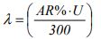 (8)
(8)
Thus an initial estimate of the actual number of passengers that will arrive in a single interval can be found by multiplying the target interval by the arrival rate of passengers as shown (9) below.
 (9)
(9)
The subscript i denotes the fact that is an initial estimate. It is worth noting that (9) is used in reference [4] as a tool to assess the actual interval at partial car loading, but not as a sizing tool.
There is no need at this stage to consider the car capacity. This can be done later when the final number of the passengers in the car has been determined.
Having arrived at an estimate for the actual number of passengers in the car, the next step is to find the corresponding round trip time. Using a classical method of calculating the round trip time [2] and [3] or using Monte Carlo Simulation [5], the value of the round trip time can be found.
The round trip time is in effect a function of the actual number of passengers if all other parameters are kept constant (such as the kinematics, number of floors, total building population, door timings, floor heights). This provides an initial value for the round trip time as shown in (10).
 (10)
(10)
From the calculated value of the round trip time, the required number of elevators can be calculated
 (11)
(11)
It is worth noting that this act of rounding up is unavoidable as a whole number of elevators can only be selected. The resultant number of elevators, L, is the nearest to the optimum as practically as possible.
Due to the process of rounding up to find the actual value of the interval will be slightly lower than the target interval, and the actual value of the handling capacity, HC%, will be slightly higher than the arrival rate, AR%.
The actual value of the interval can be found by dividing the round trip time by the number of elevators, as shown below in equation (12):
 (12)
(12)
The actual handling capacity can also be found by using equation (13) below:
 (13)
(13)
This provides an acceptable solution that satisfies Case IV discussed in the previous section. This is the optimum number of elevators required to meet the design criterion. However, it is not an optimum design regarding the required speed and car capacity. These two variables are discussed in detail in [1].
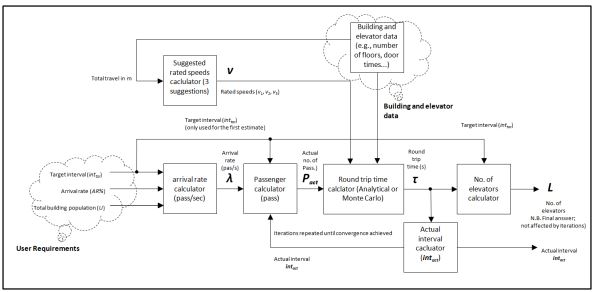
Figure 1: Block diagram showing the automated optimal design methodology.
Figure 1 shows an overview of the whole process of finding the optimum number of elevators, speed and capacity.
4. Graphical representation: The HARint Plane
The methodology described in the last section can be represented in a graphical format. The aim of the graphical representation in this case is to allow the designer to understand the effect of changes on the resulting solution, and be able to assess how far it is from the optimum solution.
In order to develop the graphical representation, a plane is presented. This plane has two axes; the x-axis represents the interval in seconds and the y-axis represents the handing capacity. Each point on the plane represents a possible solution (not necessarily an acceptable or correct one). The point representing the optimum solution, can be located by the intersection of the vertical line representing inttar and the horizontal line representing AR%, as shown in Figure 2. The plane is referred to as the HARint plane, as it contains the HC% and the AR% on the y-axis and the int on the x-axis (HCARint abbreviated to HARint).
Plotting lines of equal L (number of elevators) values and plotting lines of equal P (number of passengers) produces the HARint plane shown in Figure 2. The HARint plane can be very useful in visualising a specific solution and appreciating the optimality or otherwise of suggested solutions.
Figure 2 shows the position of the hypothetical optimum solution on the HARint plane which is the intersection point of the AR% horizontal line and the inttar vertical line. It is hypothetical because it is not achievable in practice as it requires a fractional number of elevators, L. Applying the rounding up equation (11) and then applying the iterations (as shown in reference [1]) moves the solution to the practical optimum solution (that lies on the AR% line and uses a whole number of elevators, L.
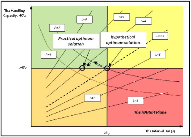
Figure 2: Hypothetical optimum solution and practical optimum solution on the HARint plane.
The use of the HARint plane shown in Figure 2 has been useful for visualising the solution, but has not been used to actually find a solution by the use of graphical methods. It might be possible to find a graphical method of finding a solution for a problem by the using the HARint plane as a solution chart (e.g., as the Smith chart is used in radio engineering and the Nichols chart is used in control systems). However, before this can be achieved, a method of normalisation needs to be introduced in order to make the HARint plane a universal tool.
5. Conclusions
A new methodology has been introduced that provides a set of rules and graphical methods that can be used to design elevator systems in buildings. The method optimises the number of elevators in the group of elevators for a building based on the user requirements of arrival rate (AR%), target interval (inttar) and the total building population (U). The methodology then optimizes the speed of the elevators and then the elevator car capacity. The method allows the user to work backwards from the actual arrival rate in the building in order to find the optimum number of elevators, instead of the trial and error method.
The methodology assumes that a method exists for accurately calculating the round trip time. Both analytical and Monte Carlo simulation methods can be used to calculate these parameters.
Due the automated and rule based nature of the methodology, it is very attractive for implementation in a software tool for the design of elevator systems.
The method has also been successfully used in teaching the principles of elevator traffic analysis to final undergraduate mechatronic engineering students at the University of Jordan. One of the main reasons for its success is that students do not possess any past experience in elevator traffic design and hence rely on the rule base and graphical methods in reaching an optimal and convergent design.
It is worth noting the analysis in this methodology has assumed a constant uniform passenger arrival process. Further work is currently being done in understanding the effect of a random arrival process on the results and the final answers.
REFERENCES
- Lutfi Al-Sharif, Ahmad M. Abu Alqumsan, Osama F. Abdel Aal, “Automated optimal design methodology of elevator systems using rules and graphical methods (the HARint plane)”, Building Services Engineering Research and Technology, published online before print 12th April 2012, doi: 10.1177/0143624412441615.
- CIBSE, “CIBSE Guide D: Transportation systems in buildings”, published by the Chartered Institute of Building Services Engineers, Third Edition, 2005.
- G.C. Barney, “Elevator Traffic Handbook: Theory and Practice”, Taylor & Francis, 2002.
- G. C. Barney, “Traffic Design” in Elevator Technology, Ellis Harwood, 1986.
- Lutfi Al-Sharif, Husam M. Aldahiyat, Laith M. Alkurdi, “The Use of Monte Carlo Simulation in Evaluating the Elevator Round Trip Time under Up-peak Traffic Conditions and Conventional Group Control”, Building Services Engineering Research & Technology, Sage Publications, August 2012 33: 319-338,
Summary of features
An Overview
Elevate is software used by designers worldwide to select the number, size and speed of elevators for all types of buildings both new and old. Elevate can also be used to demonstrate that modernizing an existing elevator installation can improve service for passengers.
Elevate’s main features.
Analysis of elevator performance in
- offices hotels hospitals shopping centres residential buildings car parks mixed use buildings airports public buildings sports and leisure complexes schools and colleges. This is achieved by techniques ranging from up peak round trip time calculations through to full dynamic simulation.
- Dynamic simulation incorporating a graphical display of elevators responding to passenger calls. For your clients, this provides a convincing visual demonstration of your proposals.
- An easy to use Windows interface. Enter basic information for a quick analysis or comprehensive data for a detailed model.
- Kinematics calculations are applied to generate accurate elevator speed profiles.
- Fully comprehensive help system and online user support.
- A facility to demonstrate your own dispatcher control system using Elevate Developer Interface. This facility is useful to test and develop dispatcher algorithms.
A more comprehensive list of features of the features included in Elevate is shown overleaf.
Warning! Elevate is an extremely powerful traffic analysis tool. However, it will not make the user an elevator traffic analysis expert. For details of training courses, recommended books and examples, please visit www.peters-research.com.
Versions
Depending on the Version of Elevate purchased, different features and functions will be available.This manual describes the full version of Elevate. For a summary of the features of other versions, please refer to the following table.
This manual describes the full version of Elevate. For a summary of the features of other versions, please refer to the following table.
Features |
Elevate |
Elevate
|
Analysis Data |
||
| Up peak analysis - assumes all people arrive at the ground floor, calculates handling capacity and interval | ü | ü |
| Enhanced up peak analysis - like up peak, but you specify the target handling capacity | ü | |
| General analysis - people can arrive at any floor - calculate up peak, two way, basement service and more! | ü | |
| General analysis for double deck elevators - all traffic flows, but with double deck elevators | ü | |
| Simulation - models the whole process of people being transported by the elevators | ü | ü* |
| Selection of control systems including conventional and destination dispatch | ü | ü* |
| Use Elevate to implement, test and demonstrate your own dispatcher algorithms with simulation | ü | |
| Select Metric or U.S. (imperial) units | ü | ü |
Building Data |
||
| Enter floor name and floor level, up to 100 floors served per group | ü | ü |
| Express zones | ü | ü |
| Unlimited entrance floors at any level | ü | |
| Single entrance floor at the lowest level in the building | ü | |
Elevator Data |
||
| Enter number of elevators, maximum 12 per group | ü | ü |
| Enter any capacity or select from standard sizes | ü | ü |
| Enter door times, or allow Elevate to choose automatically based on capacity | ü | ü |
| Enter any speed or select from standard speeds | ü | ü |
| Enter any acceleration and jerk rate or allow Elevate to choose based on speed | ü | ü |
| SELECT and SPECIFY features to help you analyse many different configurations in single run | ü | ü |
| Report options to automatically reject results that do not meet your criteria | ü | ü |
| Option for elevators in a group not to serve the same floors, e.g. basement service by only part of the group | ü | |
| Option for elevators to be specified individually, e.g. different sizes and speeds in the same group | ü | |
Passenger Data |
||
| Enter passenger loading and unloading times | ü | ü |
| Enter passenger mass | ü | ü |
| Enter capacity factor | ü | ü |
| Enter length of simulation run | ü | ü |
| Enter stair factor | ü | ü |
| Enter floor population | ü | ü |
| Passengers may arrive at any floor | ü | |
| Passengers may arrive at ground (lowest) floor only | ü | |
| Option to mix traffic types, for example passengers, goods, porter with trolley | ü | |
| Option to change intensity of traffic by time of day | ü | |
| Tools to assist fast entry of common traffic flows | ü | |
| Option to provide Elevate with a list of pasengers, and define each passenger individually | ü | |
Printed Output |
||
| Summary of data entered and results calculated - includes your job titles, company name and logo | ü | ü |
| Select toolbar button to transfer the data and results to Excel (if installed on your computer) | ü | |
Maintenance and support |
||
| Support - email (preferred) and telephone support included from date of purchase for: | 1 year | 1 year |
| Maintenance - upgrades issued to the software provided at no additional charge, from date of purchase for: | 1 year | 1 year |
| Option to renew maintenance and support with Peters Research Ltd at end of free period | ü | ü |
| Option to purchase future upgrades from Elevator World | ü | ü |
Available Formats |
||
| Software and manual available for download from internet | ü | ü |
| Software available via Internet download with printed manual | ü | |
Activating Elevate |
||
| When you purchase, we provide a key to unlock the software on our computer (plugs into USB port) | ü | |
| When you have purchased, we provide an unlocking code which unlocks the software on your computer | ü |
* indicates for up peak only
Updates
If you have a current maintenance and support agreement with Peters Research Ltd, you will be informed when updates are available. To confirm that you are using the latest version, please go to www.peters-research.com/elevate8
Developer Interface
The Elevate Developer Interface provides a way of building your own dispatcher control systems into Elevate.
The Developer Interface requires you to code your control system into a Dynamic Link Library (DLL) using Microsoft Visual C++. A sample project including a basic group control system is provided to get you started (you must own a copy of Microsoft Visual C++).
When you compile the new DLL, it is placed in the directory where Elevate is installed. Then within Elevate, select the dispatcher from the Custom options in Analysis Data. All of Elevate’s simulation and analysis options are then available to use with your dispatcher.
A sample project, DispatchW, is available in the directory where Elevate is installed.
Please note that assistance with the Developer Interface is not included in the Elevate Maintenance and Support package. Support for the Developer Interface is provided on a consultancy basis.